Human validation is not only for evaluating an LLM. It can also calibrate how the LLM is used as a scalable measurement instrument for population estimation.
An LLM can classify thousands of records at low cost, but the proportion it classifies as positive is not necessarily the true proportion in the population. By combining large-scale LLM classification with a smaller human-validated sample, we can estimate the LLM’s measurement error, correct the observed prevalence, and quantify the remaining uncertainty.
Human validation is commonly used to measure how accurately an LLM classifies individual records. However, it can serve another purpose: calibrating the population-level measurements produced by the LLM. By estimating the LLM’s sensitivity and specificity from human-validated data, we can use classical statistical methods to correct the observed positive rate. We illustrate the method with an application to job matching, where the corrected estimate helped us decide what to prioritize next.
The LLM-Positive Rate Is Not the True Prevalence
Suppose we use an LLM to classify a large dataset into two categories: positive and negative. After processing the entire dataset, the LLM classifies 40% of the records as positive.
It may be tempting to conclude that the prevalence is 40%. However, this conclusion is valid only if the LLM classifies every record correctly (or, as discussed below, if false positives and false negatives happen to offset each other exactly).
In practice, an LLM produces both false positives and false negatives:
A false positive causes the observed prevalence to be overestimated.
A false negative causes the observed prevalence to be underestimated.
The percentage classified as positive by the LLM is therefore an apparent prevalence, not necessarily the true prevalence.
The difference between the two depends on the classifier’s false-positive and false-negative rates. Consequently, model evaluation and population estimation are related but distinct problems:
A model can be useful for population estimation even if it is not perfectly accurate, provided that its measurement error can be estimated and corrected.
Human Validation as Calibration Data
Human validation is often summarized using aggregate performance metrics such as accuracy or F1 score. These metrics are useful for model evaluation, but they are not sufficient for correcting prevalence.
For prevalence correction, the most important quantities are sensitivity and specificity.
Sensitivity
Sensitivity is the probability that the LLM classifies a truly positive record as positive:
Low specificity means that the LLM incorrectly labels many negative records as positive, causing the apparent prevalence to be higher than it should be.
Together, sensitivity and specificity describe how the LLM transforms the unknown true prevalence into the observed apparent prevalence.
In this framework, the human-validated sample has two roles:
Model evaluation: measuring the LLM’s record-level classification performance.
Measurement calibration: estimating the error rates needed to correct the population-level result.
It adjusts the observed positive rate using the classifier’s sensitivity and specificity. The result is an estimate of the proportion that would have been observed if the true labels were available for the entire population.
When Does the Correction Increase or Decrease the Estimate?
The correction does not always increase the apparent prevalence. Its direction depends on the balance between false positives and false negatives.
Let FPR = 1 − Sp denote the false-positive rate and FNR = 1 − Se denote the false-negative rate. The Rogan–Gladen estimator can then be written as:
For a classifier that performs better than random, Se + Sp > 1, so the denominator is positive. Provided that the classifier makes at least some errors:
The estimate remains unchanged when the two quantities are equal.
For a perfect classifier, both error rates are zero, so \(P_t = P_a\). Intuitively, the correction increases the estimate when the expected proportion of truly positive records missed by the classifier is greater than the expected proportion of truly negative records incorrectly classified as positive:
Assuming that Pₐ, Se, and Sp are approximately independent, we omit the covariance terms. Combining the squared partial derivatives with the corresponding variances gives:
The standard error of the corrected prevalence is therefore:
\[
\mathrm{SE}(P_t) = \sqrt{\mathrm{Var}(P_t)}
\]
Under the normal approximation, an approximate 95% confidence interval is:
\[
P_t \pm 1.96 \times \mathrm{SE}(P_t)
\]
D = Se + Sp − 1 summarizes how well the classifier distinguishes positive from negative records. As D approaches zero, the correction becomes unstable: small errors in Pₐ, Se, and Sp have an increasingly large effect on the corrected estimate and its variance.
Simulation: When Does the Correction Become Unstable?
The correction depends on how well the classifier separates positive from negative records. We simulated three classifiers with the same true prevalence, Pₜ = 30%, but different values of D = Se + Sp − 1:
Strong: Se = Sp = 0.90, giving D = 0.80
Moderate: Se = Sp = 0.75, giving D = 0.50
Weak: Se = Sp = 0.55, giving D = 0.10
Each run classified 50,000 records. Sensitivity and specificity were then estimated using a balanced human-validation sample, with equal numbers of truly positive and truly negative records. For each classifier and each validation sample size from 100 to 1,000 in increments of 100, we repeated the simulation 20,000 times and applied the Rogan–Gladen correction.
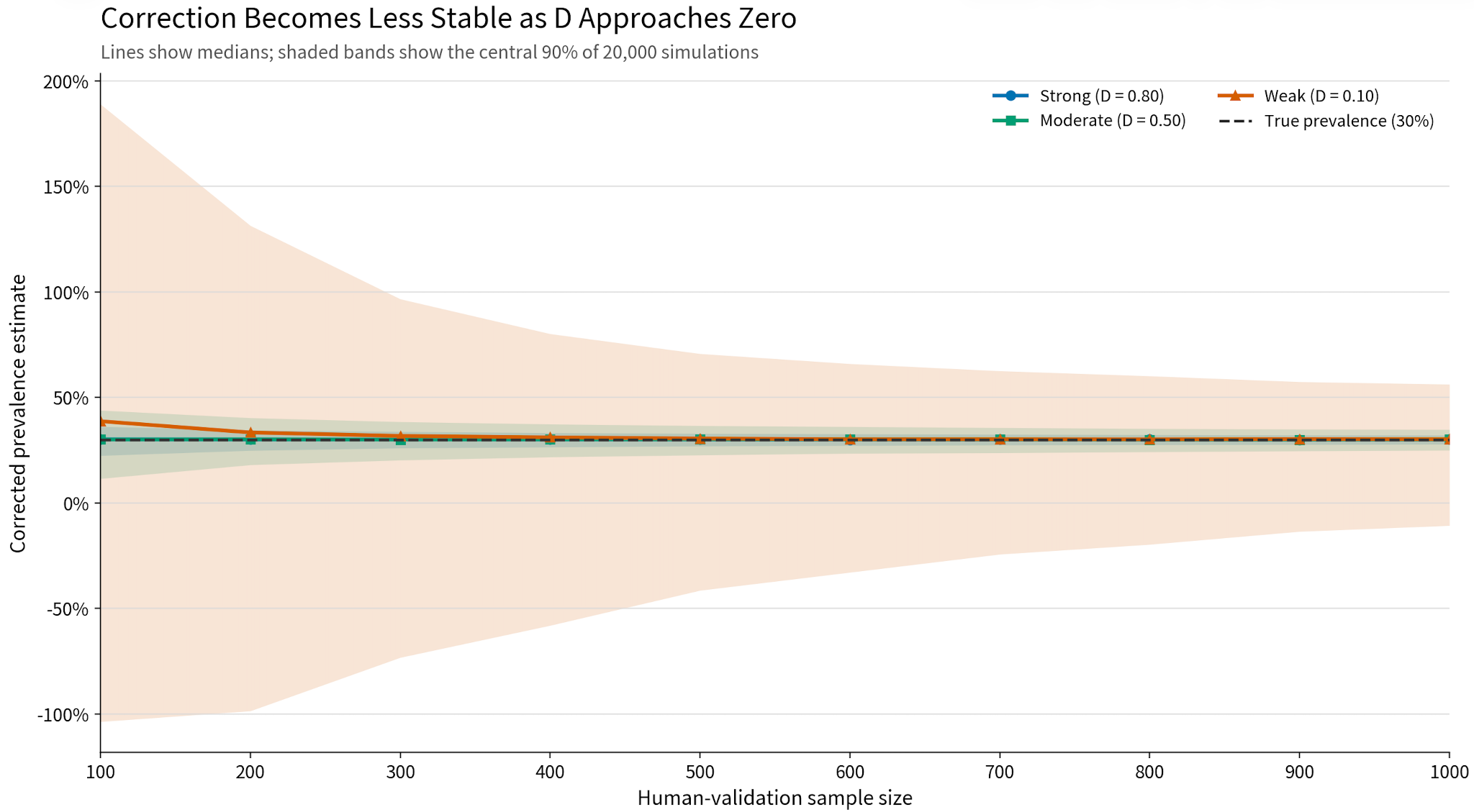
Figure 1 shows the median corrected estimate and the central 90% simulation interval. The dashed line marks the true prevalence of 30%.
Figure 1: Corrected prevalence estimates by classifier quality and human-validation sample size. Lines show median estimates; shaded bands show the central 90% simulation interval. Each sample size from 100 to 1,000 was simulated directly.
When D = 0.80, the estimates were relatively concentrated around the true prevalence even with a small validation sample. When D = 0.10, the interval remained much wider and narrowed more slowly as the validation sample grew.
A small but nonzero D does not prevent convergence, but it can amplify estimation error by a factor on the order of 1/D, and variance by a factor on the order of 1/D². A weak classifier therefore requires substantially more validation data to achieve the same precision.
Application: Opportunity Sizing for Improving Job Matching
We applied this framework to an opportunity-sizing problem in job matching. Matching systems use structured information about jobs and job seekers, such as skills, credentials, and types of work experience. We wanted to estimate how many low quality recommendations related to issues with work experience could be addressed using information the system could already represent.
The estimate helped inform a choice between two investments. High coverage would point to improving how existing information is extracted and used in matching. Low coverage would suggest that those improvements alone were not enough and that the system first needed new ways to represent the missing requirements.
We applied the LLM-based classifier to a larger dataset of about 4,000 records. Reviewing every record was not practical, so we validated about 100 records through human review. The resulting sensitivity was 73.5%, and the specificity was 77.8%. We used these estimates to correct the apparent coverage and quantify the uncertainty in the corrected estimate.
The apparent coverage was 56.4%, and the corrected estimate was 66.6% (approximate 95% CI: 47.9%–85.3%). Without the correction, our estimate would have been 10.2 percentage points lower. The correction increased the estimate because the downward effect of false negatives was larger than the upward effect of false positives. The confidence interval also made the uncertainty explicit, helping us use the estimate to inform the decision to proceed without treating it as a precise threshold.
Assumptions and Limitations
The correction is mathematically straightforward, but its validity depends on several important assumptions.
Representative human-validation sample
The human-reviewed sample should represent the population to which the correction is applied. If it contains disproportionately easy, difficult, or otherwise unusual records, the estimated sensitivity and specificity may not reflect the LLM’s performance in the broader population.
Reliable reference labels
Human labels are used as the reference standard, but they are not necessarily error-free. The target concept should be clearly defined, and reviewers should apply consistent decision criteria. Subjective tasks may require multiple reviewers or adjudication.
Sufficient validation sample size
A small human-validation sample can produce uncertain estimates of sensitivity and specificity, which in turn increases uncertainty in the corrected prevalence.
The validation sample should therefore be designed not only to evaluate record-level classification performance, but also to achieve sufficient precision in the final population estimate.
As Large Language Models (LLMs) move from research prototypes to production systems, the developers of these systems need rigorous performance evaluation. In particular, we need confidence intervals around estimates of system accuracy. However, LLMs introduce a challenge that is unusual for ML systems: they are (operationally) non-deterministic. Even with the temperature set to zero, variations in hardware, batching, and API behavior can lead to different outputs for the exact same input, and variance of model outputs can exceed variance from data sampling (Wang, 2026).
On the other hand, LLMs introduce an advantage over many other non-deterministic systems, where it can be difficult, if not impossible, to expand your data after initial collection. You cannot, for example, ask a patient to develop a disease a second time to see if the outcome changes. With LLMs, we can generate additional outputs at any time, and do so comparatively cheaply, either on the same inputs or with additional inputs.
When we create multiple LLM outputs per input, this creates a hierarchical or “clustered” data structure: we have N independent inputs, each with k correlated model runs. How should we create confidence intervals when the LLM outputs are non-deterministic? How should we make effective use of multiple LLM outputs?
The answer we propose here is the bootstrap. We simulate categorical LLM predictions and evaluate five candidate bootstrapping strategies to find out how well they correctly account for both the sampling of inputs and the non-determinism of the model itself. We’ll judge the methods based on whether their coverage matches our intended coverage, and whether they can do so with narrow confidence intervals. We then derive practical N-vs-k guidance for reducing confidence interval width, and apply the bootstrap to a well-known benchmark.
The short version. If you just want the recipe: run each of your N inputs k times, then bootstrap by resampling inputs with replacement (carrying all k runs for each chosen input), and recompute your metric on each resample; the 2.5th and 97.5th percentiles give a 95% interval. Use k = 3 or 5 if you can afford it; if the extra time and cost are a concern, run a pilot set to determine if there is sufficient benefit from the additional runs. This targets the expected accuracy of a single stochastic call, not the uncertainty of one future benchmark run or the performance of a majority-vote deployment, unless you define the metric that way. The rest of this post explains why we recommend this approach (the cluster bootstrap) over several plausible alternatives.
Assumptions
Random inputs: The N inputs are an iid (independent and identically distributed) sample from the target distribution. In particular, they are not the full population of inputs. Filtering, if any, is only done to be in line with the target distribution.
Conditionally independent outputs: Given an input, its k LLM runs are independent and identically distributed. (We assume no sequential dependencies between runs due to stateful APIs or caching).
Finite variances: We assume finite variances throughout. In practice this holds for bounded metrics like accuracy.
Bootstrap methods
We consider five variations of the bootstrap. Data is grouped (“clustered”) by N LLM inputs, and inputs are sampled with replacement to form the outer bootstrap sampling. The methods differ by k, the number of LLM calls (runs) made per input, and how those runs are used.
IID bootstrap: One LLM run per input.
Single-draw cluster bootstrap: Run k > 1 LLM calls per input. Sample the input groups with replacement. For each chosen input group, sample one of the LLM results. Bootstrap sample shape: N × 1
Cluster bootstrap: Run k > 1 LLM calls per input. Entire clusters are sampled together, with no subsampling. Bootstrap sample shape: N × k
Hierarchical bootstrap: Run k > 1 LLM calls per input. Sample the input groups with replacement. For each input group, sample the LLM runs with replacement. Bootstrap sample shape: N × k
Mode-aggregate bootstrap: Run k > 1 LLM calls per input. Aggregate the k runs into a mode, breaking ties at random. Then sample like Strategy 1, IID bootstrap. This is specific to cases where the LLM generates categorical labels, as in our simulations here. Bootstrap sample shape: N × 1
We now offer some informal reasoning (i.e., guesses) to motivate the inclusion of each of these strategies. This is not meant to be correct reasoning about the methods; it’s meant to mirror possible intuition. In fact, we’ll see later that two strategies are overly conservative and one creates an estimate of a different quantity.
In the informal reasoning below, our first goal is to include variation from LLM non‑determinism in the interval. The next consideration is budget: if we can afford multiple runs per input, how should we use them?
IID bootstrap: Our only option when we don’t have budget for multiple LLM calls. We might also prefer this strategy if we believe our model is accurate enough, or N is large enough, to not need additional LLM calls.
Single-draw cluster bootstrap: We have k > 1 LLM calls per input, to make sure we capture output variation, but only use one at a time (per selection of the input in the bootstrap sampling). In particular, we might choose this option when only one LLM call will be used per input “in production”. To reflect production usage, we elect to use only one run per input in the bootstrap.
Cluster bootstrap: With k > 1 LLM calls per input, there are a variety of reasons we might prefer this strategy: simplicity (no 2nd-level sampling), the fact that it is probably the most common type of group bootstrap, previous justification through theory and simulation (e.g., Field & Welsh, 2007), or simply the general rule that using more data is better.
Hierarchical bootstrap: Similar to the previous strategy, we know that using more data is generally better, but might worry that static clusters under-estimate the variance due to LLM non-determinism, and thus guess that bootstrapping within the k LLM calls will help us capture that variance better.
Mode-aggregate bootstrap: Combining multiple thoughts from the previous strategies with k LLM calls, we might feel that we should use only one LLM label per input, to mirror production, but somehow also use all of the k LLM calls. With the data in this case being categorical, the simplest way to include all of the LLM calls is by taking the mode.
Simulation
We simulated a simple model that predicts 4 categorical labels, with the table below representing the model’s “true” confusion matrix.
predicted
0
1
2
3
true
0
120
30
5
0
1
25
80
20
5
2
5
20
70
15
3
0
5
20
80
With this confusion matrix, the true mean accuracy is 0.70 (70%). This single-run accuracy, θ = 0.70, is our estimand: the quantity we want a confidence interval for. Keeping this target in view explains two of the results below, where a strategy goes wrong by describing a different quantity.
Data are simulated by first random sampling true labels according to the true marginal, then random sampling predicted labels given true labels. We run simulations with multiple values of the number of LLM inputs N and the number of LLM runs per input k. For each simulation, we run 2,000 trials with 5,000 bootstrap samples per trial.
For each bootstrap method, the point estimate is accuracy computed on all N × k runs collected for that method; the exception is mode-aggregate, where accuracy is computed on the N aggregated labels. A 95% confidence interval is created for each method, for each trial. The interval bounds are the 2.5th and 97.5th percentiles of the statistic recomputed on each bootstrap sample (the exception is the BCa intervals in the appendix). There are two main criteria for judging the confidence intervals:
coverage: the percentage of trials that contain the true metric value (closer to 95% is better)
the mean width of the confidence intervals (smaller is better if the coverage is good)
Each coverage figure is itself estimated from 2,000 trials, so the standard error of a coverage estimate near 0.95 is about 0.5 percentage points (√(0.95 · 0.05 / 2000)). Treating roughly two standard errors as a practical noise band, we read being off-nominal less than about 1 percentage point as possibly due to noise. For example, a single coverage value of 94.3% could indicate a real coverage issue, but could also plausibly be noise. Accordingly, we describe a method as conservative (or anticonservative) only when its coverage falls outside this band or deviates in a consistent direction across settings.
Results
N = 200 LLM inputs
First, we fix the number of LLM inputs at N = 200 and vary the number of LLM calls per input.
k=1
Coverage %
Width
IID Bootstrap
96.0
0.1266
k=2
k=3
k=5
Coverage %
Width
Coverage %
Width
Coverage %
Width
Single-draw cluster
99.6
0.1267
100.0
0.1267
100.0
0.1267
Cluster
95.0
0.0904
94.8
0.0749
95.2
0.0592
Hierarchical
98.7
0.1101
98.7
0.0954
98.9
0.0776
Mode-aggregate
95.3
0.1264
6.7
0.1085
0.0
0.0893
Fixed k, varying number of LLM inputs
N=100
N=200
N=400
k
Coverage %
Width
Coverage %
Width
Coverage %
Width
IID bootstrap
1
95.2
0.1776
96.0
0.1266
95.2
0.0895
Single-draw cluster
5
100.0
0.1788
100.0
0.1267
100.0
0.0897
Cluster
5
94.8
0.0835
95.2
0.0592
95.8
0.0420
Hierarchical
5
99.0
0.1096
98.9
0.0776
99.3
0.0550
Mode-aggregate
5
0.4
0.1255
0.0
0.0893
0.0
0.0637
Takeaways
IID bootstrap‘s coverage is near nominal, but, as might be expected when it uses less data, it has almost the widest confidence intervals.
Single-draw cluster has the widest confidence intervals, which was postulated as a necessary improvement in the informal reasoning above, but that was wrong. By keeping only one run per resampled input, its bootstrap distribution has the spread of a single-run (k = 1) estimate, even though the point estimate averages all k runs and is more precise. The interval describes more uncertainty than the estimate actually has, so it is too wide, and the coverage is extremely conservative, often maximally conservative.
Cluster has the narrowest confidence intervals. With k = 5, the width is less than half that of IID bootstrap or single-draw cluster. Field & Welsh (2007), with far fewer clusters, found that the cluster bootstrap consistently underestimated variance; in this simulation it performs well. The coverage is nearly the best, staying close to nominal across all the settings we tried.
Hierarchical has the second-narrowest intervals, but is very conservative. Compared to IID bootstrap or single-draw cluster the conservative coverage might be worthwhile given the decrease in interval width. Compared to cluster bootstrap, which has roughly 25% narrower intervals, probably not. This over-conservatism matches Field & Welsh (2007), who in a different estimation context found that the hierarchical strategy (their “two-stage bootstrap”) has “excess variation” and is inferior to the other bootstrap methods they studied.
Mode-aggregate‘s coverage is good for k = 2, though only because the math aligns with single-run estimation; coverage decreases rapidly to zero for k > 2.
Why does mode-aggregate bootstrap‘s coverage go to zero?
The mode aggregation estimates a fundamentally different model, because the mode of k will have a different accuracy rate than a single LLM call. To see this, consider a simpler situation with just two labels and a mean accuracy of 0.70 independent of inputs. With k = 3, the probability of the mode being correct is the probability of 2/3 or 3/3 correct, which is
So, the mode of k = 3 will have accuracy near 0.78, but we’re trying to estimate the single-run accuracy of 0.70. The k = 2 coverage is correct only because random tie-breaking makes the mode of two runs distributionally identical to a single run.
The aggregation idea connects to Blackwell et al. (2025), who also gather k runs for each of N inputs but aggregate in the opposite direction: they take the mean over inputs per run and use those k values to form an interval (analytically, via the t-distribution), whereas Strategy 5 takes the mode over runs per input and uses the resulting N values. Their target is also different, a prediction interval for mean benchmark performance rather than a confidence interval for single-run accuracy.
How general are these results?
Interval widths will change with the intraclass correlation ρ (defined in Choosing N and k below), but the ranking of the methods is stable. The cluster bootstrap targets the correct variance regardless of ρ. Single-draw uses less information per draw, which widens its intervals, and hierarchical’s within-cluster resampling roughly double-counts the within-input variance. Both deficits scale with 1 − ρ, so the methods converge as ρ grows toward 1. The simulation has ρ ≈ 0.025, which accentuates these differences. Mode-aggregate targets the wrong quantity at any ρ < 1.
A note on the BCa correction
A common refinement is the bias-corrected and accelerated (BCa) interval (Efron, 1987), which adjusts the percentile interval for bias and skewness. We tried it on the cluster bootstrap and it made no measurable difference for accuracy: the cluster bootstrap is already close to nominal, and with 2,000 trials (a standard error of about 0.5 percentage points) BCa changes were within Monte Carlo noise, at essentially the same width. BCa earns its keep on skewed, nonlinear metrics; we introduce, apply, and explain it in the appendix Cohen’s κ and the BCa correction, where it gives a small but consistent improvement.
Choosing N and k
The simulation results show us that, as expected, increasing either N or k leads to tighter confidence intervals. We might want to optimize further, and therefore want to have a more precise understanding of how the interval widths scale with N and k. In particular, we might use that information to know how to balance N and k with a limited budget.
Focusing on the cluster bootstrap and mean accuracy as metric, we can write the variance with separate factors depending on N and k.
We use the assumptions from the introduction, now in cluster language: clusters (inputs) are independent, observations within a cluster are conditionally iid (LLM outputs given the input), and variances are finite.
Let Yij = 𝟙[predij = actuali] be the accuracy for input i (denoted Xi) and run j, with
With the assumptions above, Yij is conditionally iid given the input Xi, and Ȳi·, the mean within cluster i, is iid given cluster independence.
where σ²B is the variance between clusters and σ²W is the variance within clusters. Since clusters are iid,
Using
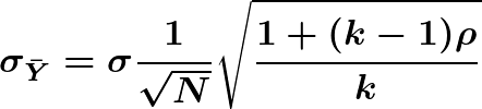
where σ² is the total population variance and ρ is the population intraclass correlation, we can write the standard deviation as
Asymptotically, interval width w is proportional to the standard deviation
These last two formulas can help us choose N and k, while typically also taking into account their relative costs. Increasing either N or k will decrease interval width, but
Hence the contribution from increasing k is capped (lower bound is √ρ), while the contribution from N is not capped. From the form of the factors, N is generally more powerful, but for many applications the easier or cheaper path will be increasing k. A similar variance decomposition underlies the N-vs-k recommendation in Miller (2024); the difference is that Miller works analytically throughout, whereas here the decomposition guides budgeting while the intervals themselves come from the bootstrap.
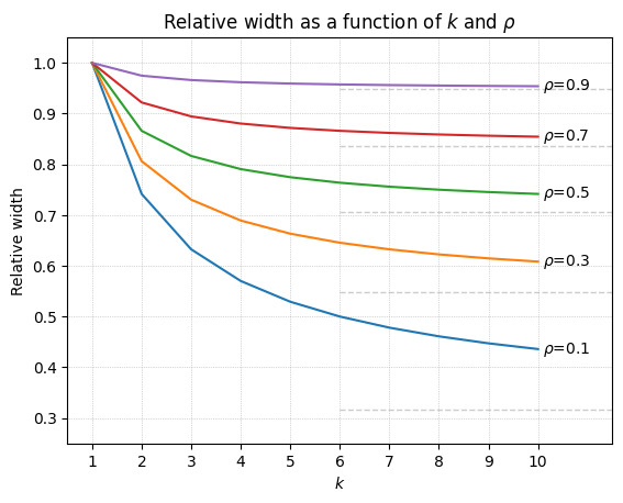
The plot below shows the factor involving k for several values of ρ.
Figure: the k-dependent factor sqrt((1 + (k-1)ρ) / k) from the width formula, plotted against the number of runs k for several values of the intraclass correlation ρ. Dashed horizontal lines mark each curve’s asymptote, √ρ. Larger ρ means a higher floor and less benefit from additional runs.
The contribution from increasing k diminishes quickly. Good initial options are k = 3 or k = 5 (assuming budget allows), and further optimization can be done from there.
Does this match the simulation? It does, closely. For the simulation’s confusion matrix the intraclass correlation works out to ρ ≈ 0.025, so the floor is √ρ ≈ 0.16: even with unlimited runs, the cluster bootstrap interval can shrink to no less than about 16% of its single-run width. (This ρ is extremely small; for comparison, our estimates from the MMLU-Pro data below range from about 0 to 0.9.) The table below shows almost perfect alignment between the width reduction predicted by the formula and the reduction actually observed for the cluster bootstrap relative to k = 1 in the N = 200 simulation.
k=2
k=3
k=5
Predicted factor
0.72
0.59
0.47
Observed factor
0.71
0.59
0.47
Use a normal approximation instead?
Miller (2024) recommends analytical confidence intervals using a normal approximation: “we regard bootstrapping as unnecessary unless a complicated sampling scheme or estimator is being used”. We agree with this quote, to some extent. We think both solutions are useful and recommend both, but if a single solution is desired, across diverse estimation tasks, we strongly recommend the bootstrap. First, unnecessary does not mean inappropriate. Bootstrap confidence intervals can be used even if we have an analytical solution. Second, the situations where the bootstrap will be the better tool are, in our experience, far from unusual:
complicated sampling schemes or metrics, as in the quote
simple metrics with skewed distributions, such as mean latency or mean cost
a missing or hard-to-derive analytical formula; this can happen even without a complicated sampling scheme or metric
paired model-model analysis with LLM outputs that are not numeric
Third, the bootstrap provides a general framework across metrics without requiring fundamental alteration. For analytical confidence intervals, changes to data collection (even if relatively simple conceptually, like switching from k = 1 to k > 1 runs per input), or introduction of a new metric, could require a new analytical solution. The bootstrap handles these situations automatically and allows us to apply corrections for skewed distributions (like the BCa correction; see the κ appendix) where the standard normal approximation falls short.
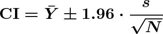
We also compared a normal approximation directly to the cluster bootstrap on the simulations above, using
where s is the sample standard deviation of the Ȳi· cluster means (iid across inputs, as discussed in the last section). For accuracy, the choice is a wash: for example, at N = 200 and k = 5, coverage is 95.2% for the cluster bootstrap versus 94.7% for the normal approximation, with mean widths of 0.0592 versus 0.0594, and the other settings match as closely. We use the cluster bootstrap because it carries over unchanged to nonlinear metrics or other situations where a normal approximation might need a custom derivation or might not exist.
Application to MMLU-Pro
Wang et al. (2024) introduced the MMLU-Pro benchmark as an iteration on MMLU with more challenging problems and with an answer set that was harder to game. Their analysis comparing model performance with Chain of Thought (CoT) instructions and without (“direct”) inspired us to look more into that comparison. Their Table 3 includes the values below. In particular, we were curious whether the smaller values represent a clear difference in model performance. In other words, if we could put confidence intervals on these numbers, how wide would they be?
% correct
Model
CoT
Direct Answer
CoT − DA
GPT-4o
72.6
53.5
19.1
GPT-4-Turbo
63.7
48.4
15.3
Phi3-medium-4k-instruct
55.7
47.5
8.2
Llama-3-8B
35.4
31.5
3.9
Gemma-7B
33.7
27.0
6.7
Performance on math and biology questions
MMLU-Pro contains questions across fourteen topics. Calculating and justifying a confidence interval across the entire benchmark could be difficult. Instead we focus on individual topics. For this exercise, we treat each topic’s questions as an iid sample from a hypothetical super-population of similarly challenging problems filtered the same way. The confidence interval then quantifies sensitivity to the specific items included.
The math subject has N = 1351 questions and biology has N = 717. Within this benchmark the items are fixed, so we can’t decrease confidence intervals by increasing N; we can only increase k.
Results are below, using k = 5 runs. We chose a set of models that a) were similar in size to the Llama 3 and Gemma models in the original table above, and b) that we could access reliably through OpenRouter. Confidence intervals were calculated through a paired cluster bootstrap, with CoT and Direct Answer responses sampled together for each iteration.
Math
Biology
% correct
CoT − Direct Answer
% correct
CoT − Direct Answer
Model
CoT
Direct Answer
Estimate
Conf. Int.
CoT
Direct Answer
Estimate
Conf. Int.
Gemma 3 12B
73.2
31.0
42.3
[39.3, 45.1]
78.1
73.4
4.7
[2.3, 7.2]
Llama 3 8B Instruct
36.8
29.2
7.6
[5.7, 9.5]
46.2
63.6
−17.4
[−19.9, −14.8]
Qwen 2.5 7B Instruct
62.9
36.2
26.7
[23.6, 29.7]
72.1
72.6
−0.6
[−2.9, +1.8]
Qwen 3 8B
90.5
91.5
−1.0
[−1.6, −0.4]
87.5
86.9
0.6
[−0.1, +1.3]
Qwen 3.5 9B
94.2
94.4
−0.2
[−0.6, +0.2]
91.5
91.0
0.4
[−0.3, +1.3]
Differences are computed before rounding.
Observations: Some of the differences here (per-subject) are larger than seen for similarly-sized models in the original table (entire benchmark). The gap for Gemma 3 12B between CoT and Direct Answer is particularly large. Several of the difference estimates are negative, which we did not see in the original table. Confidence intervals for two of the negative estimates exclude zero (Llama 3 8B Instruct on biology, Qwen 3 8B on math). Because we form ten difference intervals here, we read these exclusions descriptively rather than as formal hypothesis tests (see Exploratory vs confirmatory analysis below). Overall, the newer Qwen models performed best on both math and biology.
A note on negative results: As in Wang et al. (2024), answers are extracted with a regular expression (though ours is a bit more permissive), and a response whose answer can’t be extracted is judged incorrect. The models had varying difficulty with formatting. For example, on biology questions, 31% of Llama 3 8B Instruct’s CoT responses were misformatted (versus 2% for Direct Answer), which could account for a large part of its CoT inaccuracy.
Comparison with the original table above is difficult for a few reasons. We focus on two specific subjects rather than the entire benchmark. Also, we modified the prompts and answer extraction based on their performance on a pilot sample. So we do not directly answer whether the original table’s small gaps are real. Instead, we show something more general: with k runs per input and a paired cluster bootstrap, gaps of a few percentage points can be separated from run-to-run noise, or shown to be indistinguishable from it. More results and details are in the appendix.
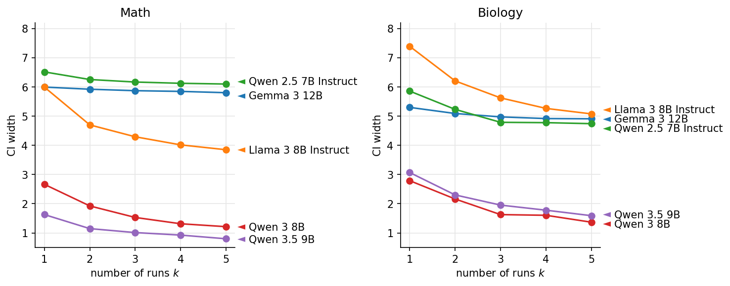
The plots below show the confidence interval width for k = 1, 2, …, 5.
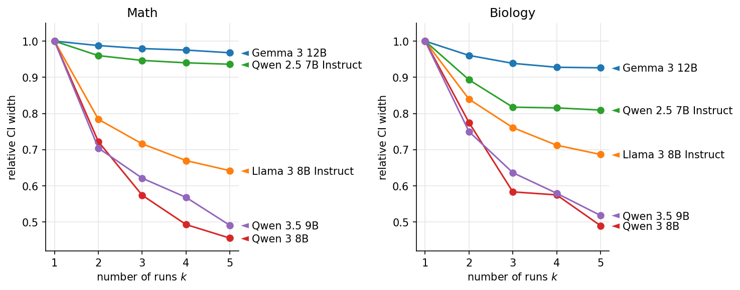
Figure: absolute width of the 95% confidence interval for the CoT − Direct Answer accuracy difference, by number of runs k, for each model (MMLU-Pro math and biology). Width shrinks with k but the gains flatten quickly, mirroring the capped-k behavior of the width formula.Figure: the same CI widths relative to their k=1 value. Each curve approaches a floor rather than continuing to zero, the empirical counterpart of the √ρ asymptote in the previous section.
Estimating ρ
We estimated ρ for the difference in correctness between CoT and Direct Answer, using the between- and within-question mean squares of a one-way ANOVA.
Math
Biology
k=5 width factor
k=5 width factor
Model
ρ
Pred.
Obs.
ρ
Pred.
Obs.
Gemma 3 12B
0.89
0.95
0.97
0.87
0.94
0.93
Llama 3 8B Instruct
0.29
0.66
0.64
0.35
0.69
0.69
Qwen 2.5 7B Instruct
0.80
0.91
0.94
0.58
0.81
0.81
Qwen 3 8B
0.02
0.46
0.46
0.00
0.45
0.49
Qwen 3.5 9B
0.07
0.51
0.49
0.17
0.58
0.52
The estimated ρ values range from about 0 to about 0.89. At the low end (as with the simulation), k has almost maximal impact (low width factor, indicating large width reduction), and at the high end it has very little impact (high width factor, minimal width reduction). On the high end, Gemma’s large ρ indicates a stable CoT advantage across runs. On the low end, Qwen 3 models’ tiny differences are mostly run-to-run noise. A couple notes: (i) ρ is a ratio of variances, and not directly a measure of consistency; the Qwen 3 models have low variance, but within-question variance accounts for much more of it than between-question variance, and (ii) Qwen 3 8B’s biology ρ is clamped at zero; the raw estimate was slightly negative, which is common when the true value is near zero.
The predicted width reduction factors match the observed bootstrap width ratios very closely in most cases, supporting the formula’s usefulness. The recommendation to start with k = 3 to 5 is partly to allow estimation of ρ, which then informs whether there is value in further runs.
Exploratory vs confirmatory analysis
We present the analysis above as exploratory. We are interested in understanding the confidence intervals broadly and in seeing how they change with increasing LLM calls per input. If we had instead been interested in making hard conclusions, e.g., hypothesis tests, then we would instead use a confirmatory analysis. In that case, we would make a few changes in particular:
set and use a single k beforehand
adjust confidence intervals for multiple comparisons (e.g., Bonferroni correction)
Limitations
While the recommended cluster bootstrap approach is robust, its application in real-world LLM evaluation involves several statistical and practical constraints:
Simulation scope: Our results will not generalize to all use cases. Custom simulations are recommended if you are unsure whether the simulations here apply to your situation.
Conditionally independent outputs: We assume that model runs are conditionally independent given the input. In practice, system-level optimizations or state could introduce correlations between runs.
Variance formula is approximate for nonlinear metrics: Our analytical budget formula (Var(Ȳ) = (σ²B + σ²W/k)/N) holds exactly for sample means like accuracy. For nonlinear metrics, the formula is a first-order approximation and should be used as a qualitative guide rather than a precise planning tool.
Independence across inputs: All strategies assume the N inputs are exchangeable. If inputs are dependent, the standard bootstrap’s assumption of independence is violated, and more advanced methods may be required.
Curated test sets: The bootstrap typically assumes inputs are a random sample from an infinite population. For fixed or curated test sets, the confidence interval should be interpreted as quantifying sensitivity to the specific items included rather than uncertainty about a wider population-level metric.
Summary and recommendations
We compared five bootstrap strategies for building confidence intervals in LLM evaluation, where a model is run k times across N inputs. Through simulations and derivations we arrived at several concrete suggestions:
Use Cluster Bootstrap: For N inputs with k runs, resampling entire clusters matched nominal coverage in our simulations while avoiding the excess width of the alternatives.
Match aggregation to your deployment: If your deployed system uses an aggregate, then aggregation produces the correct target for estimation. (In this case you might want multiple aggregates per input to reduce the estimate variance.) However, if your deployed system uses a single run, then aggregation produces the wrong target, inaccurate estimates, and potentially null coverage.
Optimize between N and k: Multiple runs (k) reduce within-input noise and are often cheaper, but their contribution is capped. Increasing the number of unique inputs (N) reduces between-input noise and its contribution is uncapped, but it is often more expensive. Start with k = 3 or k = 5 if budget allows, then use the relative costs of N and k together with the width formulas to optimize further:
For a metric that is a sample mean of per-observation outcomes, like accuracy, the first formula is exact and the second asymptotically correct. The bootstrap handles other metrics automatically, including nonlinear ones; if you want an explicit analytical dependence on N and k for a nonlinear metric, a delta-method linearization gives one.
We also demonstrated the usefulness of the cluster bootstrap on the MMLU-Pro benchmark. We created confidence intervals for comparison of accuracy with Chain-of-Thought (CoT) vs. Direct Answer prompts. Confidence intervals, and using repeated runs to construct them, can clarify whether seemingly small performance gaps are distinguishable from noise.
This work speaks to two open questions raised by Atıl et al. (2025): how to account for the instability of hosted LLM systems in business products, and how to communicate that instability to decision-makers. Bootstrap confidence intervals built from repeated runs give a concrete, quantitative answer to both.
Overall, our position is this: use bootstrap confidence intervals to put principled uncertainty around your point estimates and to apply one method across metrics and estimation contexts; narrow those intervals by creating k > 1 outputs per input.
References
Atıl, B., Aykent, S., Chittams, A., Fu, L., Passonneau, R. J., Radcliffe, E., Rajagopal, G. R., Sloan, A., Tudrej, T., Ture, F., Wu, Z., Xu, L., & Baldwin, B. (2025). “Non-Determinism of ‘Deterministic’ LLM System Settings in Hosted Environments.” In Proceedings of the 5th Workshop on Evaluation and Comparison of NLP Systems, pp. 135–148. Association for Computational Linguistics. doi:10.18653/v1/2025.eval4nlp-1.12.
Blackwell, R. E., Barry, J., & Cohn, A. G. (2025). “Towards Reproducible LLM Evaluation: Quantifying Uncertainty in LLM Benchmark Scores.” arXiv:2410.03492.
Efron, B. (1987). “Better Bootstrap Confidence Intervals.” Journal of the American Statistical Association, 82(397), 171–185. doi:10.1080/01621459.1987.10478410.
Field, C. A., & Welsh, A. H. (2007). “Bootstrapping Clustered Data.” Journal of the Royal Statistical Society: Series B, 69(3), 369–390.
Fleiss, J. L., Cohen, J., & Everitt, B. S. (1969). “Large Sample Standard Errors of Kappa and Weighted Kappa.” Psychological Bulletin, 72(5), 323–327.
Miller, E. (2024). “Adding Error Bars to Evals: A Statistical Approach to Language Model Evaluations.” arXiv:2411.00640.
Wang, S. (2026). “Measuring all the noises of LLM Evals.” arXiv:2512.21326.
Wang, Y., Ma, X., Zhang, G., Ni, Y., Chandra, A., Guo, S., Ren, W., Arulraj, A., He, X., Jiang, Z., Li, T., Ku, M., Wang, K., Zhuang, A., Fan, R., Yue, X., & Chen, W. (2024). “MMLU-Pro: A More Robust and Challenging Multi-Task Language Understanding Benchmark.” In Advances in Neural Information Processing Systems, vol. 37, pp. 95266–95290. doi:10.52202/079017-3018.
Appendix: Cohen’s κ and the BCa correction
As an additional example, we run simulations for a complex nonlinear metric, namely, Cohen’s κ. We use the same “true” confusion matrix, number of trials (2,000) and number of bootstrap iterations (5,000). The tables below show simulated confidence interval coverage for 95% confidence intervals.
Because κ is nonlinear, a ratio (po − pe)/(1 − pe), its sampling distribution can be skewed even at moderate N. A general fix is the bias-corrected and accelerated (BCa) interval (Efron, 1987), which adjusts for both bias and skewness.
The tables below include a Cluster BCa row alongside the plain cluster bootstrap so the effect of the correction is visible.
N = 200 LLM inputs
k=1
Coverage %
Width
IID Bootstrap
94.9
0.1702
Normal approx
95.0
0.1702
k=2
k=3
k=5
Coverage %
Width
Coverage %
Width
Coverage %
Width
Single-draw
99.5
0.1706
100.0
0.1707
100.0
0.1707
Cluster
94.5
0.1218
94.1
0.1008
94.3
0.0799
Cluster BCa
94.7
0.1217
94.4
0.1007
94.8
0.0797
Hierarchical
98.5
0.1482
98.5
0.1285
98.7
0.1045
Mode-aggregate
94.3
0.1701
6.6
0.1465
0.0
0.1211
Fixed k, varying number of LLM inputs
N=100
N=200
N=400
k
Coverage %
Width
Coverage %
Width
Coverage %
Width
IID bootstrap
1
94.9
0.2400
94.9
0.1702
94.5
0.1203
Normal approx
1
94.6
0.2396
95.0
0.1702
94.4
0.1204
Single-draw
5
100.0
0.2421
100.0
0.1707
100.0
0.1206
Cluster
5
93.9
0.1133
94.3
0.0799
95.4
0.0565
Cluster BCa
5
94.2
0.1130
94.8
0.0797
95.6
0.0565
Hierarchical
5
98.8
0.1484
98.7
0.1045
99.1
0.0739
Mode-aggregate
5
0.5
0.1715
0.0
0.1211
0.0
0.0860
Takeaways
Performance is similar in many ways to mean accuracy. In particular,
IID bootstrap again has the best coverage but nearly the widest intervals.
The normal approximation is very similar to the IID bootstrap: nearly the same interval widths and nearly the same coverage.
For N = 100, the cluster bootstrap and its BCa variant dip slightly below nominal for κ (93.9 and 94.2), the only clearly sub-nominal case; otherwise they perform nearly as well as IID bootstrap, with the narrowest intervals.
The main difference to call out is BCa. Unlike for accuracy, where the cluster bootstrap was already at nominal and BCa made no reliable difference, the cluster bootstrap runs slightly below nominal for κ, and BCa nudges coverage up by roughly +0.2 to +0.5 percentage points at every N we tried. Each individual change is within the Monte Carlo noise, but the consistency across settings makes it credible.
For the best overall combination of coverage and interval width, use the cluster bootstrap; for nonlinear metrics, add the BCa correction. A note of caution, though: BCa estimates its bias and acceleration terms from the same data (the acceleration through a block-level jackknife), so those corrections are noisiest exactly in the small-N, high-skew regime where the correction matters most.
Normal approximation for Cohen’s κ
For k = 1, a normal approximation is available using the delta-method-derived large-sample standard error for κ̂ from Fleiss, Cohen, and Everitt (1969), computed from the estimated cell probabilities of the confusion matrix:
Unlike mean accuracy, there is (as far as we know) no clean extension to k > 1, so this formula is restricted to k = 1.
The results above show that the normal approximation matches the IID bootstrap almost exactly in both coverage and width. However, the cluster bootstrap needed no new derivation to handle either k > 1 or the switch from accuracy to κ.
Appendix: More results and details for MMLU-Pro
Models and versions
Models were accessed through OpenRouter using pinned IDs:
Display name
OpenRouter ID
Released
Gemma 3 12B
google/gemma-3-12b-it
Mar 2025
Llama 3 8B Instruct
meta-llama/llama-3-8b-instruct
Apr 2024
Qwen 2.5 7B Instruct
qwen/qwen-2.5-7b-instruct
Sep 2024
Qwen 3 8B
qwen/qwen3-8b
Apr 2025
Qwen 3.5 9B
qwen/qwen3.5-9b
Mar 2026
All calls were made with temperature 0 and a 16,384-token limit. We did not pin OpenRouter providers, so run-to-run variation includes both within-provider non-determinism and any variation from provider routing.
Introductory prompt text
Version 1
Version 2
CoT
The following are multiple choice questions (with answers) about {category}. Think step by step and then output the answer in the format of “The answer is (X)” at the end.
The following are six multiple choice questions about {category}. The first five are solved for you, with answers given. The last one is a test question for you to solve. Think step by step and then output the answer in the format of “The answer is (X)” where X is the correct or best letter choice. If you do not end your answer in this format, or if you do not select exactly one choice, your answer will be judged as incorrect.
Direct Answer
The following are multiple choice questions (with answers) about {category}. Reply with “The answer is (X)” where X is the correct letter choice.
The following are six multiple choice questions about {category}. The first five are solved for you, with answers given. The last one is a test question for you to solve. Reply with “The answer is (X)” where X is the correct or best letter choice. If you do not end your answer in this format, or if you do not select exactly one choice, your answer will be judged as incorrect.
Version 1 is similar to Wang et al. (2024), inferred in part from their GitHub repo. The main difference between CoT and Direct Answer is the addition of “Think step by step” in this introductory text (bolded here for saliency).
Version 2 was used for our study. In a pilot sample on math, we observed 4-5 percentage points higher accuracy overall with version 2. Llama 3 8B Instruct had the largest gain, roughly 15 percentage points better. Performance decreased only for Qwen 3 8B on CoT, with accuracy about 3% worse.
Apart from the change to introductory text, the prompts are created as in Wang et al. (2024).
Answer extraction
Similar to Wang et al. (2024), we used two regex patterns to find the prompt’s final answer. We attempted to be very explicit about requiring an exact answer format in our Version 2 prompt above, but we allowed for some variation. Our regex patterns are similar to Wang et al. (2024), but a bit more permissive.
We first attempted to match the first pattern. We used the last match if any was found (assuming the last match would be the “final” answer). If no match was found, we used the second pattern, again using the last match found if any. If no match was found, the response is marked as wrong. This differs from the original benchmark code, where a random answer is inserted when no match is found. The table below shows the percent of responses where a match was found, in the “Correct Format” column.
Math
Biology
Model
Prompt
Correct Format
Correct Answer
Correct Format
Correct Answer
Gemma 3 12B
CoT
98.5%
73.2%
99.7%
78.1%
Direct Answer
100.0%
31.0%
100.0%
73.4%
Llama 3 8B Instruct
CoT
86.1%
36.8%
69.1%
46.2%
Direct Answer
91.5%
29.2%
97.8%
63.6%
Qwen 2.5 7B Instruct
CoT
83.9%
62.9%
99.8%
72.1%
Direct Answer
99.2%
36.2%
100.0%
72.6%
Qwen 3 8B
CoT
97.5%
90.5%
100.0%
87.5%
Direct Answer
98.5%
91.5%
100.0%
86.9%
Qwen 3.5 9B
CoT
99.3%
94.2%
99.9%
91.5%
Direct Answer
99.6%
94.4%
99.9%
91.0%
Average
95.4%
64.0%
96.6%
76.3%
Overall, a high percentage of responses had the correct format (i.e., had extractable answers). Llama 3 8B Instruct had the most issues returning the correct format, especially on CoT. It had incorrect format for 14% of math CoT responses and 31% of biology CoT responses. Note Llama 3’s gap in performance for biology aligns well with its gap in formatting. It seems reasonable to guess that removing the formatting gap might also remove the performance gap.
Reasons for incorrect format
Across several models, responses occasionally reached the maximum allowed number of tokens, which was set at 16,384. Thus an answer that would be formatted correctly could be cut off by that limit. Judging by the table above, this was infrequent enough to be a minor issue.
Llama 3 and Qwen 2.5 both had difficulty following the instructions for answer formatting for math with CoT. We observed responses where the letter answer was given, but not in a format parseable by our regular expression, or an answer was given but without using the answer letter (e.g., a boxed numeric value). In biology CoT, Llama 3 had a more fundamental difficulty: in most failing responses, it acknowledged the task and indicated it was ready for the question, not recognizing that the question had already been given.
Recommendation and ranking systems power many of the most important experiences on large internet platforms. Yet the models that run in production are rarely the largest models we can train. They are usually compact, latency-sensitive supervised models that need to score huge candidate sets for millions of users under tight cost constraints.
That creates a practical tension:
We want to use rich, long-term behavioral histories and modern deep learning.
We still need millisecond-level latency for high-traffic ranking, recommendation, and bidding systems.
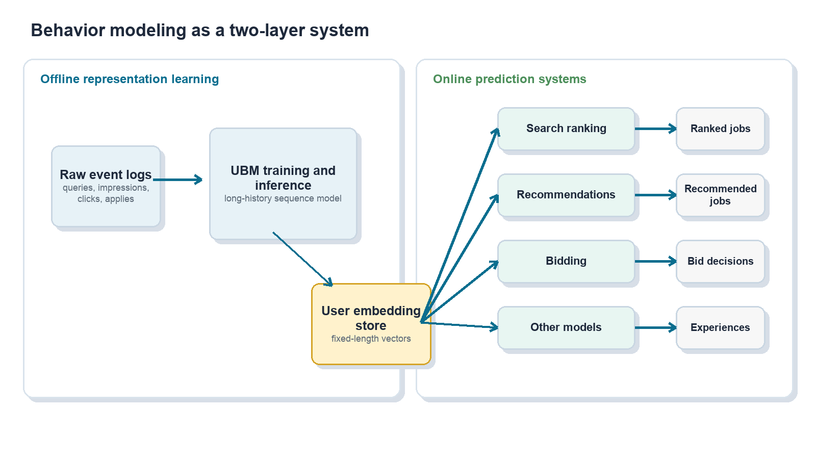
This post describes how we addressed that tension in job search by building a user behavior modeling system, or UBM, that learns from long-tail user histories offline and distills them into compact user embeddings that many online models can consume.
At a high level, UBM:
Mines long-term user behavior with deep sequence models.
Distills each user’s history into a fixed-length embedding.
Makes that embedding available through a feature store.
Lets existing production models use the embedding with minimal serving changes.
Produces consistent multi-percent lifts across several high-traffic surfaces.
The core idea is simple: do the expensive sequence modeling once, offline, and reuse the resulting user representation many times online.
Why long-tail user behavior is hard to use directly on production
For a job platform, understanding job seekers is central to matching the right people with the right roles. A user’s history can include many signals across the hiring journey:
Search queries, including titles, keywords, companies, and locations.
Job impressions and clicks.
Saves and bookmarks.
Apply starts and completions.
Employer responses and downstream outcomes.
In principle, this history is highly valuable. In practice, traditional tabular modeling often forces several compromises.
First, we keep fixed-length windows, such as the most recent K actions, and discard the rest. Second, we aggressively aggregate sequences into statistics such as “top title words” or “fraction of clicks in industry X.” Third, we rely on one-hot or sparse features that lose semantic similarity across titles, skills, companies, and industries.
Those simplifications can distort user intent. Consider a job seeker who once applied to civil engineering roles, later explored medical software trainer roles, and eventually settled into senior account management. A naive aggregation over title tokens might over-weight the word “software” and push the system toward software engineering recommendations, even though the user’s recent and consistent behavior points elsewhere.
At the same time, directly serving stacked sequence models over raw per-impression history did not fit our existing production infrastructure, where high-traffic systems need to score large candidate sets within strict latency and cost budgets.
We needed a system that could let large models learn from raw sequences offline, then feed a distilled representation into the compact online models that already power production traffic.
Behavior modeling as sequence modeling
We model user behavior as sequences, much like sentences in natural language processing:
Sequences of jobs seen, clicked, saved, or applied to, with metadata such as title, location, salary, company, and category.
Sequences of search queries and their attributes.
Other contextual events are ordered over time.
Sequence models are useful here because they can denoise long histories, capture temporal structure, and learn semantic relationships between jobs, queries, and users. The serving constraint shapes the architecture: a large offline model reads long histories and emits a user embedding, while many small online models consume that embedding as an ordinary dense feature.
Conceptually:
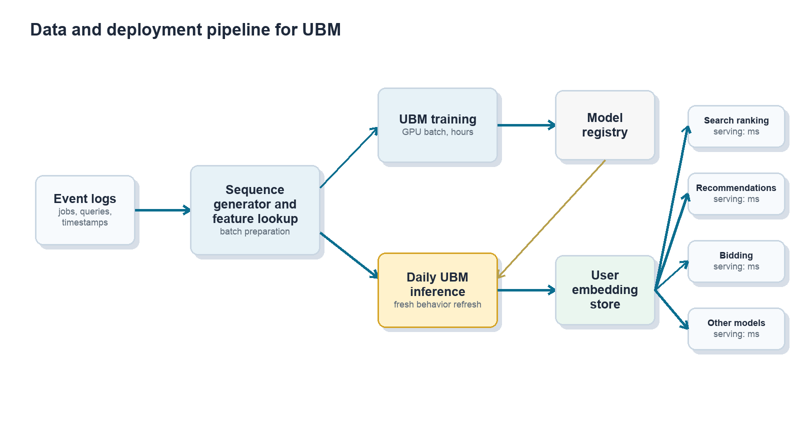
Heavy sequence modeling happens offline; light scoring happens online many times.
Architecture: from raw events to user embeddings
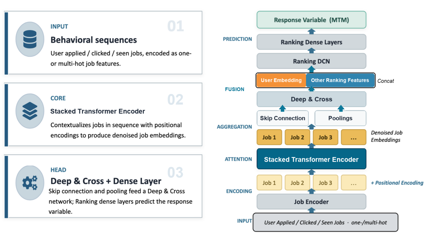
1. Encode jobs and events
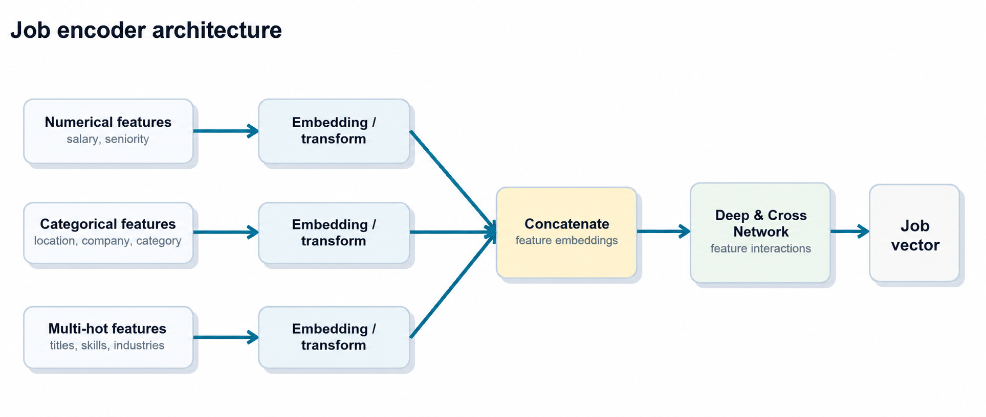
The first step is to encode individual jobs and events into dense vectors. Each job contains multiple feature types:
Numerical features, such as salary and seniority signals.
Categorical features, such as location, job category, and company.
Multi-hot features, such as normalized titles, skills, and industries.
Each feature type is mapped into embeddings. Those embeddings are concatenated and passed through a Deep & Cross Network, producing a compact job embedding that captures both linear and non-linear feature interactions.
The same job encoder is reused across behavior streams so that all sequences live in a consistent embedding space.
2. Build behavior sequences
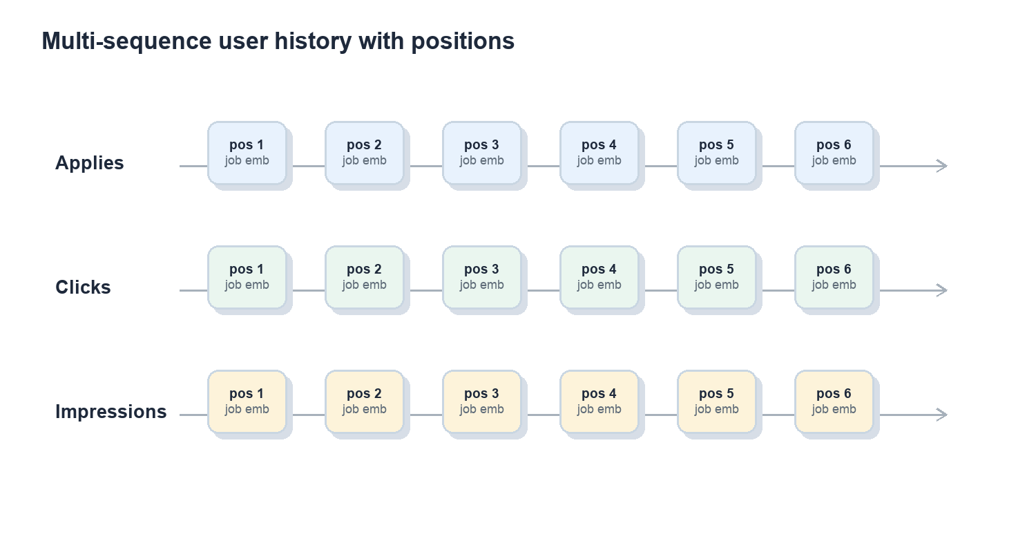
In practice, we have gone through two generations of behavior encoders: an earlier multi-sequence design and our current unified single-sequence design. In the first production version of UBM, user history was naturally treated as multi-channel: each action type was represented as a separate time-ordered sequence of job embeddings:
User U
Apply: [job_a1, job_a2, …, job_aN]
Click: [job_c1, job_c2, …, job_cM]
Impression: [job_i1, job_i2, …, job_iK]
Each sequence includes positional encodings so the model can reason about recency, order, and temporal patterns instead of treating user history as an unordered set.
3. Denoise long histories with self-attention
Long histories are noisy. People explore, change direction, compare roles casually, or click jobs that are only loosely relevant. The sequence model needs to separate durable intent from one-off behavior.
In the multi-sequence version, each action-specific sequence is passed through multi-head self-attention or transformer encoder blocks. The model re-weights each event in the context of the full sequence. Consistent patterns are amplified; isolated or off-topic events are down-weighted.
After attention, we pool the denoised sequence and combine it with skip connections from the original embeddings. Another Deep & Cross block then produces a per-sequence embedding, such as an “apply history embedding” or “click history embedding.”
4. Evolve from multi-sequence fusion to a unified event timeline
Different actions carry different information:
Apply history is strong but sparse.
Click and impression history is weaker but dense, and captures exploration.
Saves, ignores, and other actions add nuance.
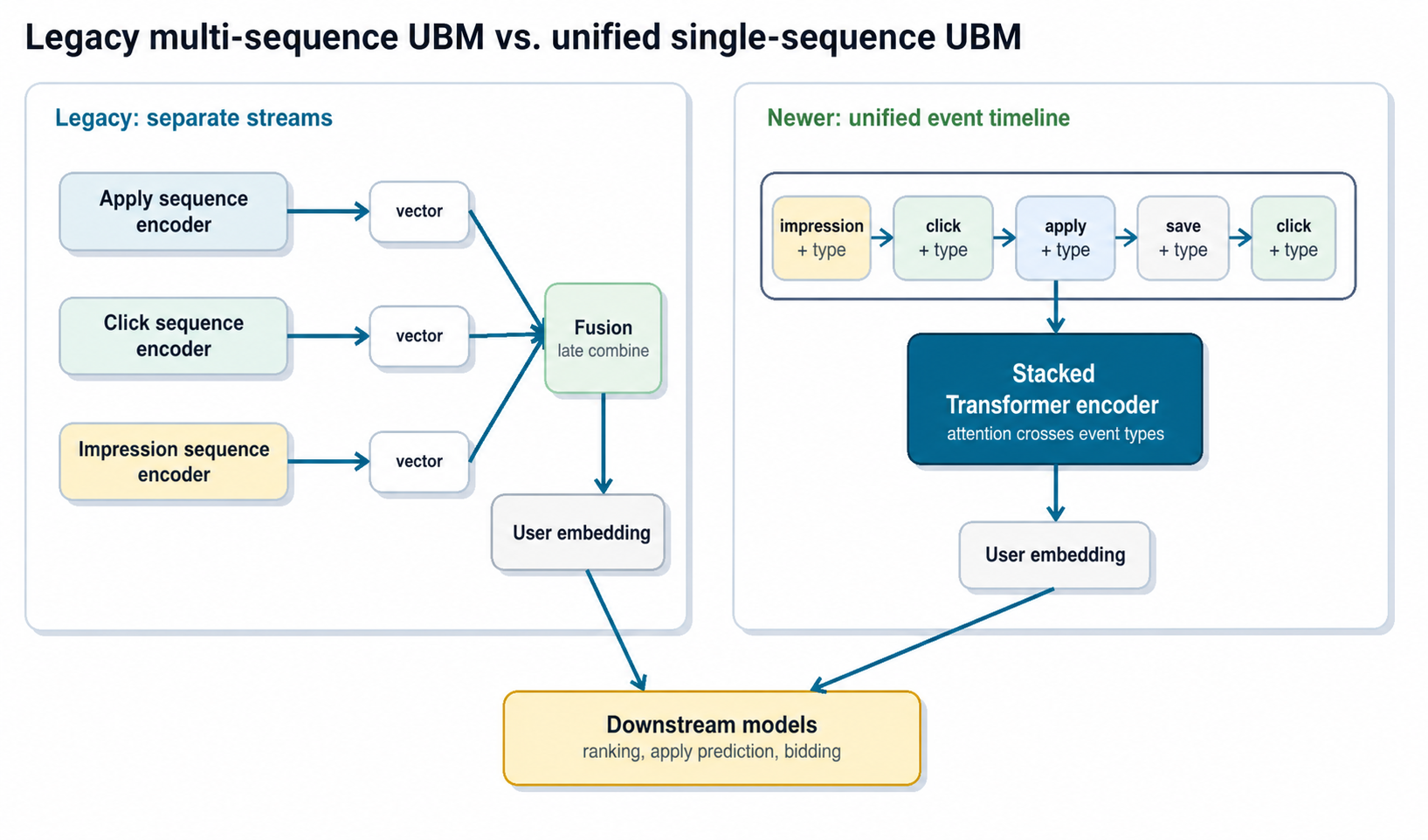
The first generation of UBM learned separate encoders for different behavior streams, then concatenated or fused their outputs into a single user history embedding. That design worked well: the final vector was expressive enough to capture long-term structure, but small and fixed-length enough for downstream models to consume cheaply.
More recently, we found that we could simplify the architecture and improve results by moving to a single-sequence design:
Merge all events, such as applies, clicks, impressions, and saves, into one unified timeline sorted by time.
Add an explicit event-type embedding to each step so the model knows whether the event was an apply, click, impression, or another action.
Let one transformer stack attend over the unified sequence instead of maintaining separate stacks per action type.
This design has two practical advantages.
First, it simplifies the model and pipeline. There is one sequence encoder to train, maintain, and monitor. Adding a new event type becomes a matter of adding a new event-type representation, rather than wiring a new encoder into the model and downstream feature pipeline.
Second, it gives attention layers direct access to cross-event patterns. The model can learn transitions such as “impression to click to apply” inside one timeline, rather than relying on separate per-action summaries that are fused only after each stream has already been compressed. This also follows a broader trend in modern sequence modeling: expose as much raw event data as possible and minimize hand-crafted aggregation, so the model can discover these patterns directly from first-hand signals.
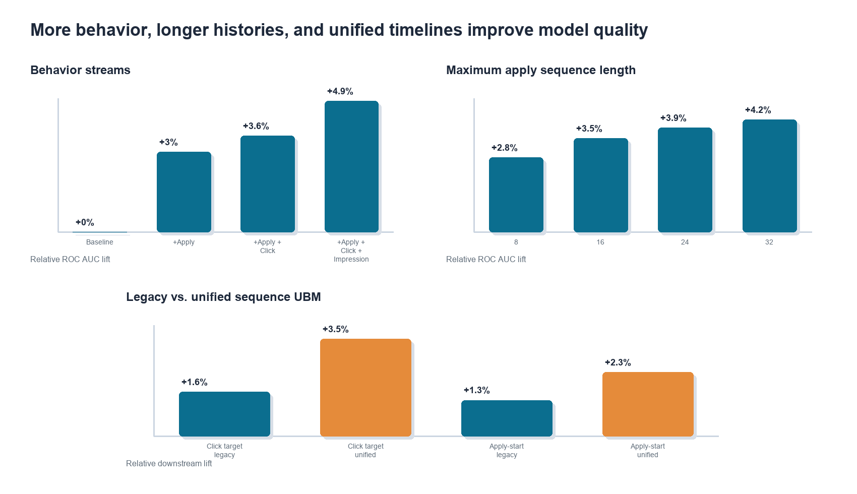
In a large downstream model, switching from the legacy multi-sequence UBM to the unified single-sequence behavior model roughly doubled the relative ROC-AUC gain over the no-UBM control model on several targets. For example, in one experiment the relative ROC-AUC improvement over control on the CTR target went from about +1.6% to +3.5%, and on the apply-start target from about +1.3% to +2.3%, using the same downstream architecture and data.
Training and serving at scale
Offline training
Training the offline sequence model is challenging because each user can interact with hundreds of jobs, and each job can have many attributes. Naively materializing all joins between users, events, and job attributes would inflate the training table by hundreds of times (each example references hundreds of jobs), turning a TB-scale dataset into PB-scale. Keeping jobs in a side table and doing cached GPU lookups instead cuts the effective data volume by hundreds of times and gives us over 100× faster training in internal benchmarks, since dense array lookups are exactly what GPUs are good at.
The offline model is trained on months of historical data and updated periodically; in the unified single-sequence version, the same pipeline emits one chronologically sorted event stream per user, with event-type features attached to each step.
Daily embedding refresh
The model itself does not need to be retrained every day, but user behavior changes continuously. To keep embeddings fresh:
We run daily batch inference with the latest user histories.
The model remains fixed during that refresh cycle.
Input sequences slide forward as new events arrive.
Updated embeddings are written to a feature store for downstream consumers.
In practice, the offline model can remain useful for months between retraining cycles, while daily inference keeps user representations current enough for production ranking and recommendation.
Online consumption by many models
Downstream ranking, recommendation, and bidding models treat the UBM embedding as one more input feature. This is the key to make the system deployable:
Production models do not need to be rewritten as transformers.
Existing tabular models can be retrained with an additional dense feature.
Online serving cost changes only modestly because the heavy sequence modeling has already happened offline.
This “one producer, many consumers” pattern also improves consistency. Multiple surfaces share a common view of user intent instead of each team rebuilding its own local behavior features.
How much does this help?
Offline model quality
On an offline apply-prediction benchmark, we compared a strong baseline model with traditional features against the same model augmented with UBM embeddings. Adding more behavior streams improved ROC AUC consistently in the multi-sequence version:
We also found that longer histories helped. Extending maximum sequence length from 8 to 32 events showed monotonic gains, with diminishing returns as the sequence length increased. While figure 7 only shows this early sweep up to 32 steps, our current production UBM models already use sequence lengths up to 256 events, and we are actively exploring longer contexts as we scale up infrastructure.
The newer unified single-sequence model kept the same operational pattern but improved downstream lift by letting the model attend across event types directly:
Click-based target: roughly +1.6% with legacy multi-sequence UBM, improving to about +3.5% with unified single-sequence UBM.
Apply-start rate: roughly +1.3% with legacy multi-sequence UBM, improving to about +2.3% with unified single-sequence UBM.
These results support two intuitions:
More behavior channels matter because different actions contain complementary signals.
Long-tail history matters because the model can learn to denoise behavior instead of relying on hand-truncated windows.
Event order across behavior types matters because job search intent often emerges through transitions, not isolated action streams.
Impact on high-traffic job surfaces in production
The more important question is what happens in production.
Because the same embedding can be reused across many models, the impact compounds across surfaces. In production experiments, adding UBM features produced consistent gains in recommendation quality, apply efficiency, and monetization metrics.
Surface
Relative lift
Jobseeker Email Recommendations
Application rate +5.24%
Jobseeker Homepage recommendations
Application rate +2.04%
Employer Resume Search
NDCG@10 +2.89%
Employer Candidate Recommendations
Employer Acceptance rate +1.64%
Across downstream models, the UBM embedding is often ranked as a top-1 or top-2 feature by importance, consistent with the observed business impact.
Extending beyond user behavior
Once the infrastructure existed for user behavior, the same pattern became useful elsewhere in the marketplace.
Employer behavior modeling applies analogous techniques to employer interactions with candidates. Those embeddings can feed sourcing, ranking, and bidding systems.
Knowledge graph and item embeddings offer another extension. Graph-based methods can encode relationships between jobs, companies, skills, and users, and those representations can be combined with sequence-based UBM and employer behavior embeddings.
The broader pattern is reusable: train richer representation models offline, distill them into compact embeddings, and expose them as shared features for production systems.
Design trade-offs and lessons learned
The offline-online split is worth it
Splitting the model into a heavy offline encoder and light online consumers sacrifices some optimality. For example, attention is not conditioned on the exact target job at scoring time. But the latency and cost benefits are large, and the resulting system is much easier to deploy across many production models.
Sequence modeling beats hand-built aggregates
Raw sequences across behavior types are more expressive than handcrafted features such as “percentage of clicked jobs in industry X.” The model learns which events to emphasize, which to down-weight, and how behavior changes over time. The single-sequence design extends this lesson: preserving cross-event order can be more valuable than summarizing each action stream independently and fusing later.
Staleness is manageable, but must be monitored
Embeddings do not need to be retrained every week, but they do need operational monitoring. Useful diagnostics include offline ROC AUC and log loss, online KPIs, feature distribution checks, and day-over-day cosine similarity of user embeddings to catch pipeline anomalies.
Centralized embeddings reduce duplicated effort
A shared embedding producer lets multiple product teams benefit from the same representation learning investment. It also reduces duplicated local behavior features and makes user understanding more consistent across surfaces.
Where we are heading next
UBM is now a foundation layer for many ranking, recommendation, and bidding systems, but several directions remain active:
Richer unified sequence modeling across search, browse, apply, and off-platform signals.
Joint user-employer modeling so both sides of the marketplace can be represented together.
Tighter integration with retrieval and approximate nearest-neighbor search.
Better use of behavior embeddings as context for large language models in hiring workflows.
Standardized tooling and observability so downstream teams can adopt embeddings safely.
The goal is straightforward: use long-term behavioral data to make job search and hiring more relevant, while staying within the real-world constraints of large-scale production systems.