Key Idea
Human validation is not only for evaluating an LLM. It can also calibrate how the LLM is used as a scalable measurement instrument for population estimation.
An LLM can classify thousands of records at low cost, but the proportion it classifies as positive is not necessarily the true proportion in the population. By combining large-scale LLM classification with a smaller human-validated sample, we can estimate the LLM’s measurement error, correct the observed prevalence, and quantify the remaining uncertainty.
Human validation is commonly used to measure how accurately an LLM classifies individual records. However, it can serve another purpose: calibrating the population-level measurements produced by the LLM. By estimating the LLM’s sensitivity and specificity from human-validated data, we can use classical statistical methods to correct the observed positive rate. We illustrate the method with an application to job matching, where the corrected estimate helped us decide what to prioritize next.
The LLM-Positive Rate Is Not the True Prevalence
Suppose we use an LLM to classify a large dataset into two categories: positive and negative. After processing the entire dataset, the LLM classifies 40% of the records as positive.
It may be tempting to conclude that the prevalence is 40%. However, this conclusion is valid only if the LLM classifies every record correctly (or, as discussed below, if false positives and false negatives happen to offset each other exactly).
In practice, an LLM produces both false positives and false negatives:
- A false positive causes the observed prevalence to be overestimated.
- A false negative causes the observed prevalence to be underestimated.
The percentage classified as positive by the LLM is therefore an apparent prevalence, not necessarily the true prevalence.
The distinction can be expressed as follows:
Apparent Prevalence
\[\text{Apparent prevalence} = \frac{\mathrm{TP} + \mathrm{FP}}{\mathrm{TP} + \mathrm{FN} + \mathrm{TN} + \mathrm{FP}}
\]
True Prevalence
\[\text{True Prevalence} = \frac{\mathrm{TP} + \mathrm{FN}}{\mathrm{TP} + \mathrm{FN} + \mathrm{TN} + \mathrm{FP}}
\]
The difference between the two depends on the classifier’s false-positive and false-negative rates. Consequently, model evaluation and population estimation are related but distinct problems:
A model can be useful for population estimation even if it is not perfectly accurate, provided that its measurement error can be estimated and corrected.
Human Validation as Calibration Data
Human validation is often summarized using aggregate performance metrics such as accuracy or F1 score. These metrics are useful for model evaluation, but they are not sufficient for correcting prevalence.
For prevalence correction, the most important quantities are sensitivity and specificity.
Sensitivity
Sensitivity is the probability that the LLM classifies a truly positive record as positive:
\text{Sensitivity} = \frac{\mathrm{TP}}{\mathrm{TP} + \mathrm{FN}}
\]
Low sensitivity means that the LLM misses many truly positive records, causing the apparent prevalence to be lower than it should be.
Specificity
Specificity is the probability that the LLM classifies a truly negative record as negative:
\text{Specificity} = \frac{\mathrm{TN}}{\mathrm{TN} + \mathrm{FP}}
\]
Low specificity means that the LLM incorrectly labels many negative records as positive, causing the apparent prevalence to be higher than it should be.
Together, sensitivity and specificity describe how the LLM transforms the unknown true prevalence into the observed apparent prevalence.
In this framework, the human-validated sample has two roles:
- Model evaluation: measuring the LLM’s record-level classification performance.
- Measurement calibration: estimating the error rates needed to correct the population-level result.
Correcting the Observed Prevalence
Let:
\[\begin{aligned}
P_t &:\quad \text{True prevalence} \\
P_a &:\quad \text{Apparent prevalence} \\
\mathrm{Se} &:\quad \text{Sensitivity} \\
\mathrm{Sp} &:\quad \text{Specificity}
\end{aligned}
\]
An LLM-positive record can arise in one of two ways:
- The record is truly positive and is correctly classified as positive.
- The record is truly negative but is incorrectly classified as positive.
Using the law of total probability:
\[P_a = \mathrm{Se} \times P_t + (1 – \mathrm{Sp}) \times (1 – P_t)
\]
Rearranging this equation gives:
\[P_a = (\mathrm{Se} + \mathrm{Sp} – 1)P_t + (1 – \mathrm{Sp})
\]
Solving for \(P_t\):
\[P_t = \frac{P_a – (1 – \mathrm{Sp})}{\mathrm{Se} + \mathrm{Sp} – 1}
\tag{1}
\]
This is known as the Rogan–Gladen estimator.
It adjusts the observed positive rate using the classifier’s sensitivity and specificity. The result is an estimate of the proportion that would have been observed if the true labels were available for the entire population.
When Does the Correction Increase or Decrease the Estimate?
The correction does not always increase the apparent prevalence. Its direction depends on the balance between false positives and false negatives.
Let FPR = 1 − Sp denote the false-positive rate and FNR = 1 − Se denote the false-negative rate. The Rogan–Gladen estimator can then be written as:
P_t = \frac{P_a – \mathrm{FPR}}{1 – \mathrm{FPR} – \mathrm{FNR}}
\]
Subtracting the apparent prevalence \(P_a\) gives:
\[P_t – P_a = \frac{P_a \times (\mathrm{FPR} + \mathrm{FNR}) – \mathrm{FPR}}{1 – \mathrm{FPR} – \mathrm{FNR}}
\]
For a classifier that performs better than random, Se + Sp > 1, so the denominator is positive. Provided that the classifier makes at least some errors:
- The correction increases the estimate when:
P_a > \frac{\mathrm{FPR}}{\mathrm{FPR} + \mathrm{FNR}}
\]
- The correction decreases the estimate when:
P_a < \frac{\mathrm{FPR}}{\mathrm{FPR} + \mathrm{FNR}}
\]
- The estimate remains unchanged when the two quantities are equal.
For a perfect classifier, both error rates are zero, so \(P_t = P_a\). Intuitively, the correction increases the estimate when the expected proportion of truly positive records missed by the classifier is greater than the expected proportion of truly negative records incorrectly classified as positive:
\[\mathrm{FNR} \times P_t > \mathrm{FPR} \times (1 – P_t)
\]
When the false-positive contribution is larger, the correction decreases the estimate instead.
Quantifying Uncertainty
The uncertainty of the corrected prevalence depends on three quantities:
- The apparent prevalence, Pₐ
- The sensitivity, Se
- The specificity, Sp
For readability, we omit hats from the estimated quantities in this section.
Let:
- n be the number of records used to estimate the apparent prevalence.
- n₊ = TP + FN be the number of truly positive records in the human-validation sample.
- n₋ = TN + FP be the number of truly negative records in the human-validation sample.
Under binomial sampling, their approximate variances are:
\[\mathrm{Var}(P_a) \approx \frac{P_a \times (1 – P_a)}{n}
\] \[
\mathrm{Var}(\mathrm{Se}) \approx \frac{\mathrm{Se} \times (1 – \mathrm{Se})}{n_{+}}
\] \[
\mathrm{Var}(\mathrm{Sp}) \approx \frac{\mathrm{Sp} \times (1 – \mathrm{Sp})}{n_{-}}
\]
The corrected prevalence is a nonlinear function of these three estimates. Let:
\[D = \mathrm{Se} + \mathrm{Sp} – 1
\]
To approximate the variance, we apply the first-order delta method. The relevant partial derivatives are:
\[\frac{\partial P_t}{\partial P_a} = \frac{1}{D}
\] \[
\frac{\partial P_t}{\partial \mathrm{Se}} = -\frac{P_a + \mathrm{Sp} – 1}{D^2} = -\frac{P_t}{D}
\] \[
\frac{\partial P_t}{\partial \mathrm{Sp}} = \frac{\mathrm{Se} – P_a}{D^2} = \frac{1 – P_t}{D}
\]
Assuming that Pₐ, Se, and Sp are approximately independent, we omit the covariance terms. Combining the squared partial derivatives with the corresponding variances gives:
\[\mathrm{Var}(P_t) \approx \frac{1}{D^2} \times \left\{ \mathrm{Var}(P_a) + P_t^2 \times \mathrm{Var}(\mathrm{Se}) + (1 – P_t)^2 \times \mathrm{Var}(\mathrm{Sp}) \right\}
\]
The standard error of the corrected prevalence is therefore:
\[\mathrm{SE}(P_t) = \sqrt{\mathrm{Var}(P_t)}
\]
Under the normal approximation, an approximate 95% confidence interval is:
\[P_t \pm 1.96 \times \mathrm{SE}(P_t)
\]
D = Se + Sp − 1 summarizes how well the classifier distinguishes positive from negative records. As D approaches zero, the correction becomes unstable: small errors in Pₐ, Se, and Sp have an increasingly large effect on the corrected estimate and its variance.
Simulation: When Does the Correction Become Unstable?
The correction depends on how well the classifier separates positive from negative records. We simulated three classifiers with the same true prevalence, Pₜ = 30%, but different values of D = Se + Sp − 1:
- Strong: Se = Sp = 0.90, giving D = 0.80
- Moderate: Se = Sp = 0.75, giving D = 0.50
- Weak: Se = Sp = 0.55, giving D = 0.10
Each run classified 50,000 records. Sensitivity and specificity were then estimated using a balanced human-validation sample, with equal numbers of truly positive and truly negative records. For each classifier and each validation sample size from 100 to 1,000 in increments of 100, we repeated the simulation 20,000 times and applied the Rogan–Gladen correction.
Figure 1 shows the median corrected estimate and the central 90% simulation interval. The dashed line marks the true prevalence of 30%.
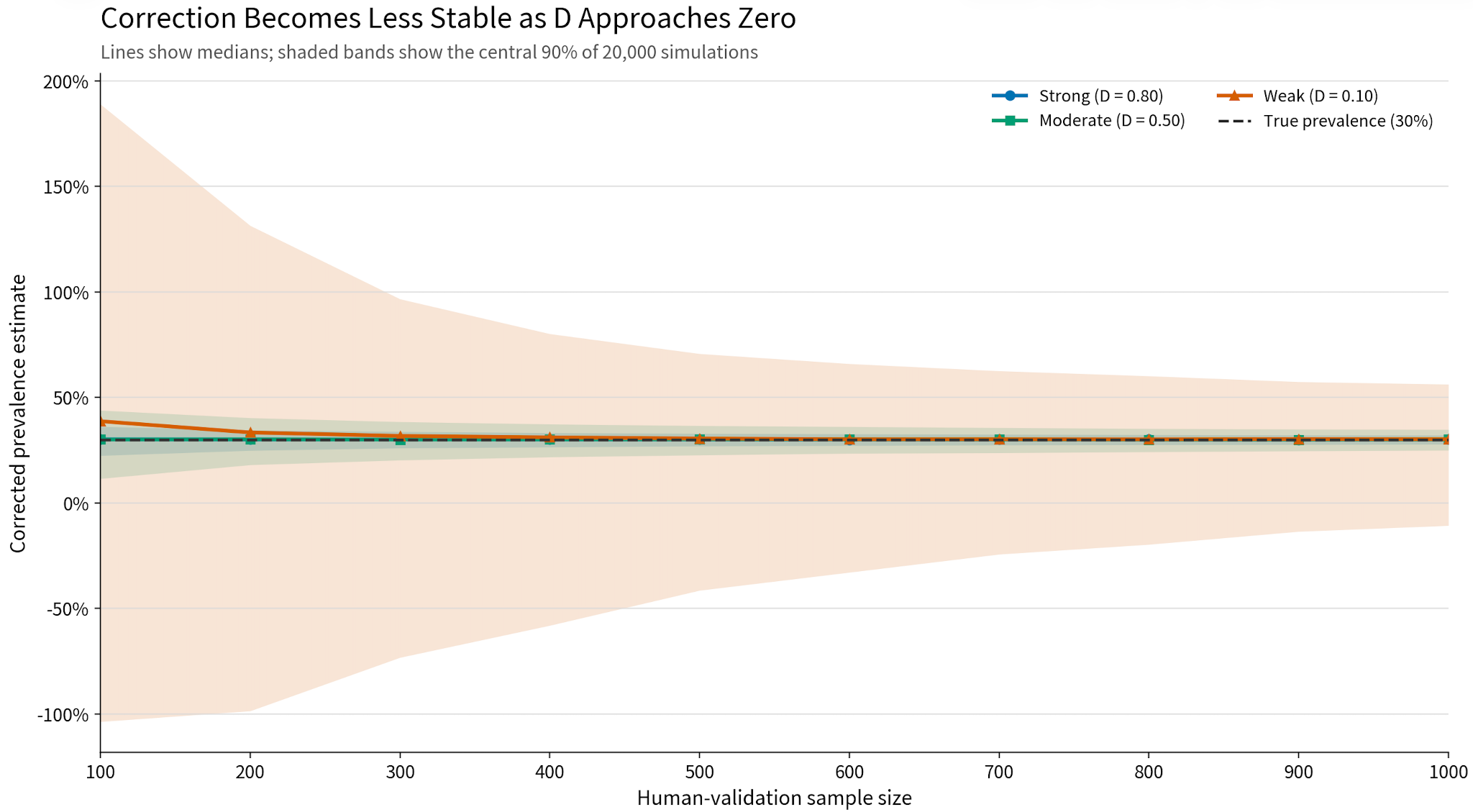
When D = 0.80, the estimates were relatively concentrated around the true prevalence even with a small validation sample. When D = 0.10, the interval remained much wider and narrowed more slowly as the validation sample grew.
A small but nonzero D does not prevent convergence, but it can amplify estimation error by a factor on the order of 1/D, and variance by a factor on the order of 1/D². A weak classifier therefore requires substantially more validation data to achieve the same precision.
Application: Opportunity Sizing for Improving Job Matching
We applied this framework to an opportunity-sizing problem in job matching. Matching systems use structured information about jobs and job seekers, such as skills, credentials, and types of work experience. We wanted to estimate how many low quality recommendations related to issues with work experience could be addressed using information the system could already represent.
The estimate helped inform a choice between two investments. High coverage would point to improving how existing information is extracted and used in matching. Low coverage would suggest that those improvements alone were not enough and that the system first needed new ways to represent the missing requirements.
We applied the LLM-based classifier to a larger dataset of about 4,000 records. Reviewing every record was not practical, so we validated about 100 records through human review. The resulting sensitivity was 73.5%, and the specificity was 77.8%. We used these estimates to correct the apparent coverage and quantify the uncertainty in the corrected estimate.
The apparent coverage was 56.4%, and the corrected estimate was 66.6% (approximate 95% CI: 47.9%–85.3%). Without the correction, our estimate would have been 10.2 percentage points lower. The correction increased the estimate because the downward effect of false negatives was larger than the upward effect of false positives. The confidence interval also made the uncertainty explicit, helping us use the estimate to inform the decision to proceed without treating it as a precise threshold.
Assumptions and Limitations
The correction is mathematically straightforward, but its validity depends on several important assumptions.
Representative human-validation sample
The human-reviewed sample should represent the population to which the correction is applied. If it contains disproportionately easy, difficult, or otherwise unusual records, the estimated sensitivity and specificity may not reflect the LLM’s performance in the broader population.
Reliable reference labels
Human labels are used as the reference standard, but they are not necessarily error-free. The target concept should be clearly defined, and reviewers should apply consistent decision criteria. Subjective tasks may require multiple reviewers or adjudication.
Sufficient validation sample size
A small human-validation sample can produce uncertain estimates of sensitivity and specificity, which in turn increases uncertainty in the corrected prevalence.
The validation sample should therefore be designed not only to evaluate record-level classification performance, but also to achieve sufficient precision in the final population estimate.